Keywords: Linear region, viscoelastic, rheology, DMA
RH107
Background
This note will describe the linear viscoelastic region (LVR) and how to determine the LVR in oscillatory experiments for the purpose of obtaining quality data. All aspects of the LVR discussed in this note are general to viscoelastic samples, including (but in no way limited to) polymers, foods, gels, creams, pastes, slurries, emulsions, and inks.
The Linear Visceolastic Region and its Importance
The linear viscoelastic Region (LVR) is important in rheology and dynamic mechanical analysis because the viscoelastic parameters of the material are strain independent below a critical strain. Small strain experiments interrogate the sample without changing the microstructure. Reported values of the glass transition, moduli, complex viscosity, and tan(δ) typically assume the measurement was conducted within the LVR unless otherwise explicitly stated. Often, for the typical experiment, determining the exact end of the LVR is not as critical as simply avoiding strains that are clearly outside the LVR while generating enough torque or force to create quality data at all temperatures, frequencies, and states of the material. This note will detail how to determine the critical strain quantitatively in two ways but the user should be able to recognize the end of the linear region from the drop in the storage modulus or where the stress-strain relationship becomes clearly nonlinear.
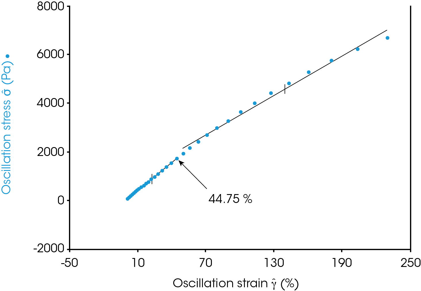
The linear viscoelastic region (or simply the “linear region”) of a material is defined by a linear relationship between the complex stress and oscillatory strain. The complex stress will be referred to simply as “stress” and the oscillatory strain will be “strain.” This note will discuss the LVR in the context of oscillatory measurements. The linear region has no lower bound, however, at sufficiently high strains the stress response becomes nonlinear. This relationship is shown in Figure 1 for a molten polymer. Below the strain of ~44% the stress has a linear relationship with the strain. Above ~44% the stress increases less than linearly with strain. This strain is referred to as the critical strain and it marks the end of the linear region for this material at a given frequency and temperature.
Methods to Determine the Critical Strain
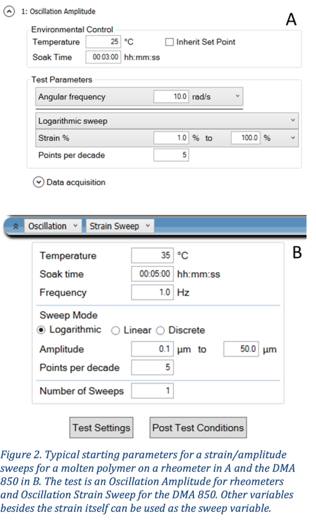
A strain sweep (TRIOS experimental setup in Figure 2) is used to determine the LVR and critical strain in oscillatory measurements. It is important that the material is stable and not changing during the sweep. The sample should be stable at the measurement temperature and equilibrated for at least 5 minutes.
Often, when dealing with a new material, a bit of trial and error are associated with setting the strain range. It is important to note that there is no consequence to setting the strain too low except noisy data. Always start low and sweep to a higher strain. High strain will likely change the microstructure of a material and it will take time for that structure to recover if it recovers at all.
A strain sweep does not always need to be performed for every frequency and temperature because the lowest critical strain will usually be at the lowest temperature and highest frequency, particularly for polymers. When determining the LVR for a temperature ramp, run a strain sweep at the coldest temperature. When determining the LVR for a frequency sweep, choose a frequency close to the highest frequency.
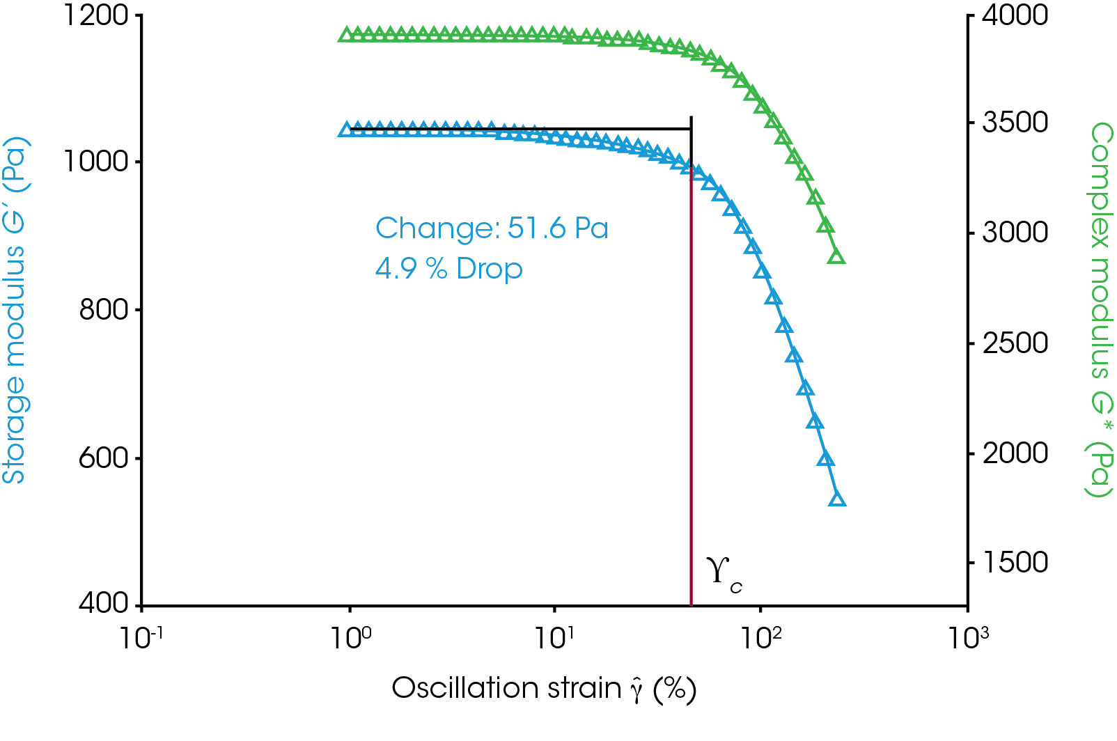
The complex modulus is the stress normalized by the strain and is mathematically the slope of the stress vs strain line in the linear region. The phase angle determined from the oscillatory measurements can be used to calculate a storage modulus which is very sensitive to the structure of a viscoelastic material. The complex and storage moduli have a constant value and do not change with the applied strain within the linear region. As the strain increases outside the LVR the structure of the material is changed because of the high strain oscillation and a drop in the storage modulus is observed (Figure 3). The critical strain marked on the figure corresponds to a ~5% drop in the storage modulus from the average of the plateau. Alternatively, the user can do an onset analysis in which a line is fit to the plateau region and the drop-off region. The intersection of these lines can be used as the critical strain.
Figure 1 shows a transition from the linear region but does not show a very obvious transition. The transition can be made obvious in TRIOS if the log of the complex stress is plotted vs the log of the strain. The derivative of the log – log relationship between stress and strain is equal to one in the linear region and drops below one outside the linear region (Figure 4). The reason for this relationship is shown as follows: Equation 1 can be used to describe a linear relationship:
y = mx n+b
When n =1 for a line. Replace y, x, and m with our rheological variables σ, γ, and G* respectively for a single frequency and temperature of a stable material:
σ = G* γ n
Where σ is the stress, G* is the complex shear modulus, γ is the strain, and n is the index. The stress-strain relationship of a material has no stress with no applied strain, so the intercept, b, is always zero and it is not included. If we take the log of both sides:
Log(σ) = Log(G* γ n )
Expand the right side using the rules of logarithms:
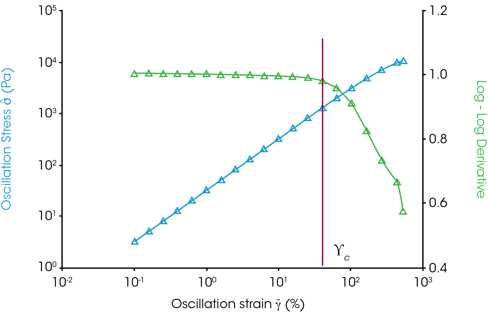
Equation 2 is the stress strain relationship with n = 1 in the linear region. Taking the log of both sides of the equation gives equation 4, a line that has a slope equal to the index, n, and intercept of log(G*). If we calculate the derivative of the log of stress vs log of strain plot we get the index, n, at each point and can see where it begins to deviate from one. Figure 4 shows the log(σ) vs log(γ) in blue with the derivative calculated by TRIOS in green. The derivative drops below 1 at the critical strain marked on the plot. The only input a user has is determining how much of a deviation from 1 constitutes nonlinear but this is largely academic. The end of the linear region is very clear in this plot.
As a side note: the stress at the critical strain can be considered a critical stress. It is often much easier to work in terms of strain so the LVR is usually characterized by the critical strain instead. This critical stress can be used as a yield stress in some applications.
Strain and Noise
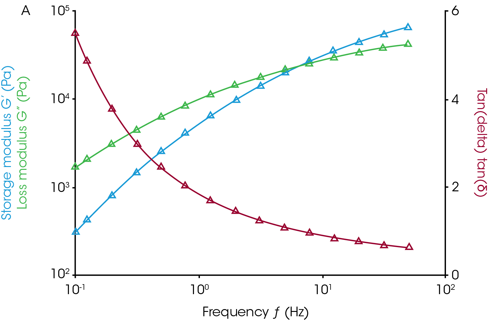
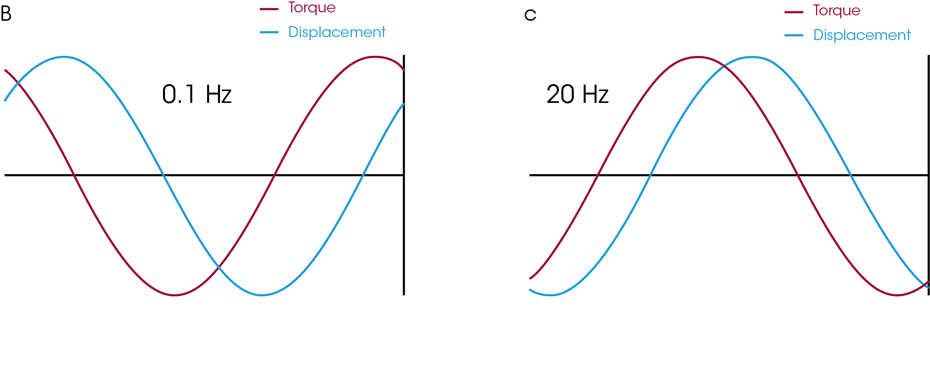
It is instructive to see what good and bad data look like. High quality “good data” in the LVR look like the waveforms in Figure 5 (b and c.) These waveforms are collected for each datapoint in the frequency sweep. The strain is set at 1%, which is well below the critical strain (15%) at high frequencies. Both the displacement and torque signal are smooth and sinusoidal. These waveforms are saved by default in any instrument running TRIOS and aid greatly in troubleshooting data. Users can easily tell which signal is noisy and adjust either the strain or tools/geometry appropriately.
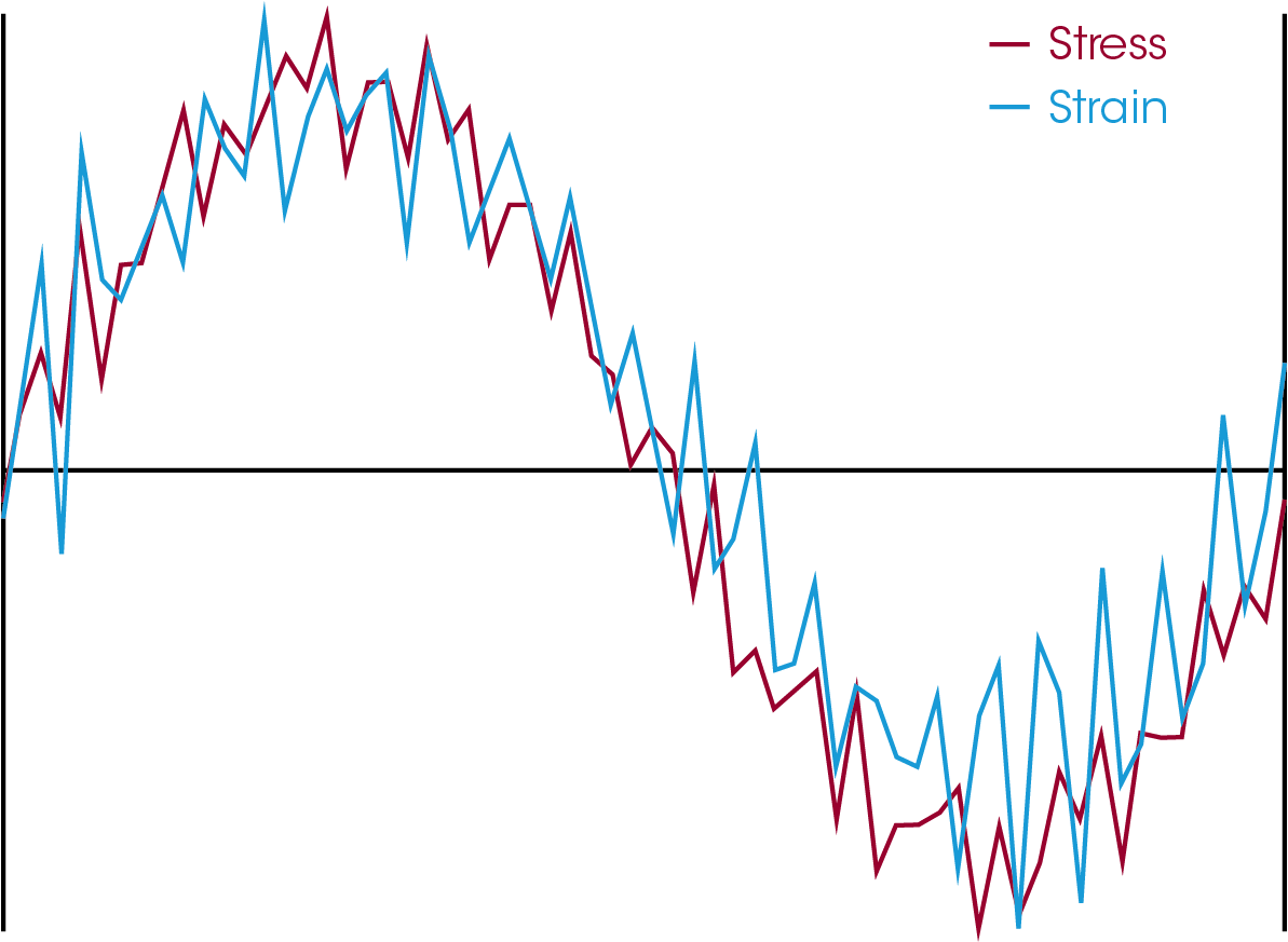
Poor quality data can be generated when the strain is set too low. The data in Figure 6 were collected on a DMA 850 at a low displacement of 100 nm. The stress and strain curves are both noisy, likely due to environmental noise such as ventilation, foot traffic, and other sources of vibrations. Many vibrational environmental effects can be mitigated by separating the instrument from the source of vibration and placing the instrument on a marble table. These mitigation efforts work for rheometers and DMA instruments. There will always be some noise and increasing the strain can increase the torque or force which will increase signal above the noise. A strain/amplitude sweep provides the information the user needs to determine where good data is being generated as well as the end of the LVR. Users should change the measuring geometry if good data cannot be generated within the LVR. Use a different clamp or sample size to increase stiffness in DMA experiments. Rheometers have multiple plate and cone sizes, as well as the Couette system to increase the torque generated.
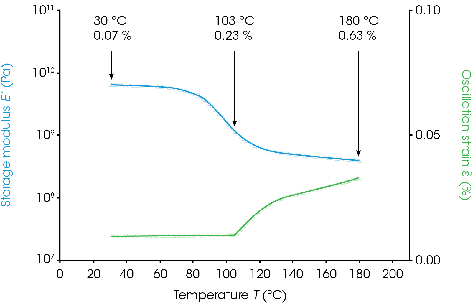
Minimum torque (DHR), minimum force (DMA850/Q800), and auto-strain (RSA-G2 and ARES-G2) are experimental settings that can be used to automatically increase the strain a small amount in order to maintain the minimum signal levels above the noise but not increase above the critical strain. Figure 7 shows the use of auto-strain on a PETE (Polyethylene Terephthalate) film sample. Once the sample softens significantly in the transition region the strain is increased slightly to maintain a minimum force set in the procedure. The linear region at three temperature points was determined in prior experiments. The oscillation strain stayed well below the labelled critical strain in the glassy region (30 °C), the transition region (103 °C) and in the rubbery plateau (180 °C).
The critical strain typically increases with temperature in polymer systems, so it is often acceptable to set a lower bound to the force/torque and allow the strain to increase as a material softens significantly. It is advisable to run a strain or amplitude sweep at the lowest and highest temperature of the experiment to get an idea of what strain is required for quality data and what the critical strain is.
Conclusions
This note has described how to determine the linear viscoelastic region and critical strain for oscillatory measurements. These methods are general and apply to nearly any material. The critical strain is important because data above the critical strain do not represent the material at equilibrium and change the structure that the experiment aims to measure. When the strain is set too low the quality of data can suffer if not enough signal (displacement, torque, or force) is generated.
Acknowledgement
This application note was written by Kevin Whitcomb, Ph.D, Application Engineer at TA Instruments.
Click here to download the printable version of this application note.

